

Over the past few months, I have received numerous requests for information regarding the topic of advanced analytics. Many of these requests center around the concept of how to register a new data function using TIBCO Spotfire. Although this capability has been available in Spotfire for quite some time, it appears that many people are now discovering it for the first time as they approach business problems that are increasingly more complex.
Given the renewed interest in this topic, I have decided to post an example of how to register a new data function in Spotfire. I encourage you to use the data and code files included at the bottom of this post to follow along. I believe you will find that the process is much simpler than you might expect. Once you master this process, an entire new vista of advanced analytics will be available to you.
Problem description: Register a new TERR data function that will allow any user to fit a Loess Smoothing function to a set of data. In this example, I assume you are using the Spotfire Analyst Client with the Spotfire Server up and running.
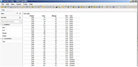
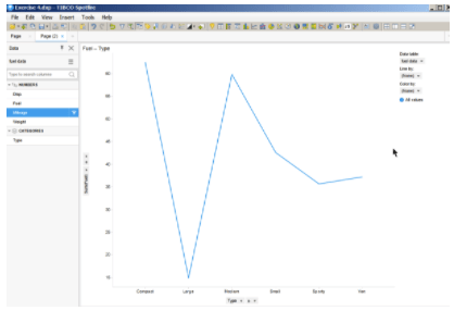
1. Open the file named “fuel_data.dxp”. This dataset contains information about various types of cars, their type, weight, displacement, fuel, and gas mileage.
2. Create a simple line chart to show the relationship between car weight and gas mileage. Clearly, there is a relationship between weight and mileage. Heavier cars have lower gas mileage.
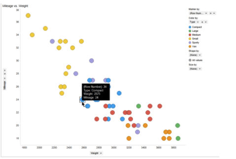
3. After reviewing the scatter plot, we decide that it might be helpful to draw a smoothing curve through the points to help see overall trends or relationships between these two variables. We decide to create a new Data Function that will calculate a Loess Smoothing Function.
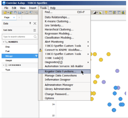
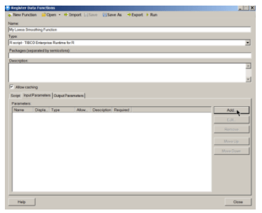
Begin by selecting “Register Data Functions” from the Tools menu.
4. Give your new Data Function a name. In this example, I have named it “My Loess Smoothing Function”. You can name it anything you wish. Enter the TERR code shown below (see TERR_Script.txt).
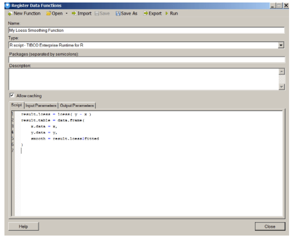
result.loess = loess( y ~ x )
result.table = data.frame(
x.data = x,
y.data = y,
smooth = result.loess$fitted
)
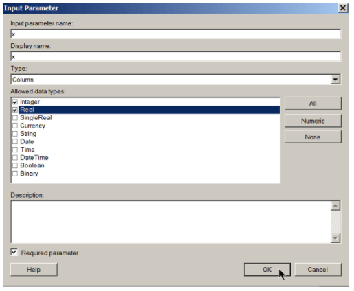
5. Click the “Input Parameters” tab and then click “Add”.
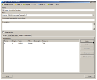
6. Complete the dialog box as shown below. Click “OK”. This action sets up the x-axis parameter that will be fed into the function.
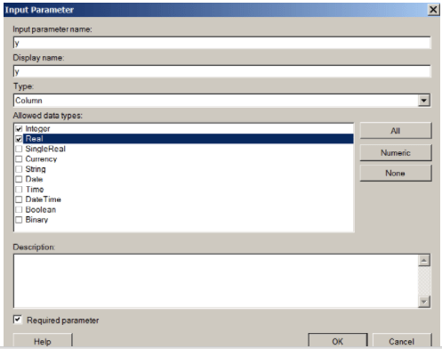
7. Click the “Input Parameters” tab and then click “Add”.
8. Complete the dialog box as shown below. Click “OK”. This action sets up the y-axis parameter that will be fed into the function.
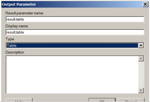
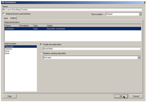
9. Click the “Output Parameters” tab and then click “Add”.
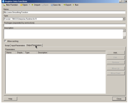
10. Complete the dialog box as shown. This will set up the result output table that will contain the smoothed data function.
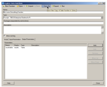
11. Click the “Save As” button. Select the directory to put your new Data Function in. Click “Save”. When finished, click the “Close” button. You have now created a new Data Function which can be used at any time to plot a smoothing function over top of a set of data.
12. Open a new page in Spotfire. Add a line chart as shown.

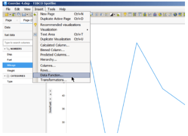
13. Select “Data Function” from the “Insert” menu.
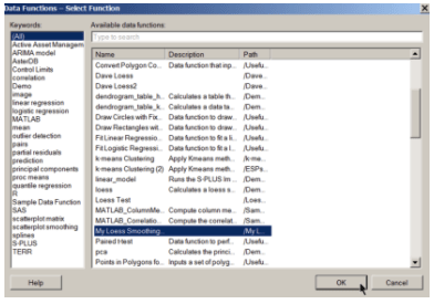
14. Find your new Data Function by name. Highlight it and then click “OK”.
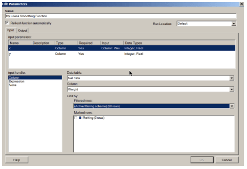
15. Map the “x” variable to the weight column in your dataset as shown below. Be sure to check the “Refresh function automatically” and “(Active filtering scheme)” options as shown.
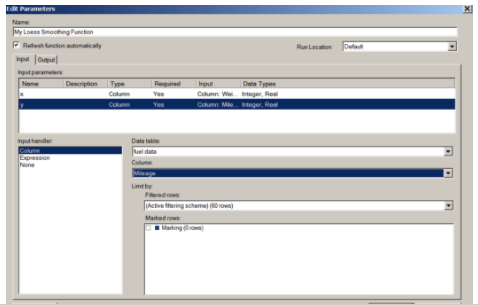
16. Map the “y” variable to the mileage column in your dataset as shown below. Be sure to check the “Refresh function automatically” and “(Active filtering scheme)” options as shown.
17. Click the “Output” tab and then map the “result.table” output as shown. When finished click “OK”.
18. Back on the line chart page, change the data source for the line chart to be “result.table”. This is the smoothing function output you just created when you inserted the data function.

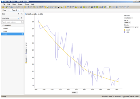
19. Using the Data panel place the “Smooth” and “y.data” values on the vertical axis. Place the “x.data” on the horizontal axis.
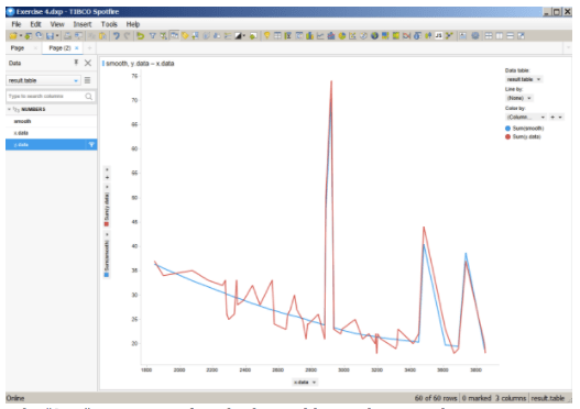
20. Remove the “Sum” aggregation from both variables on the vertical axis.
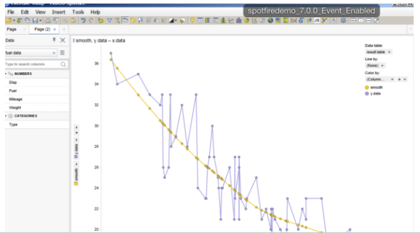
21. Go to “Properties” for the line chart. From the “Appearance” option choose to display markers. You will now see the original mileage and weight data with a Loess Smoothing Function plotted over top. As you filter data from the original “Fuel Data” data table the function will automatically recalculate and the graph will be updated in real time.
Congratulations, you just registered your first Data Function!

Try this and TIBCO Spotfire’s other great features in a free software trial. Start yours today.


